Wednesday, December 28, 2011

How to plot using pstricks(3) --- plot a data file

The second data plotting command is "\dataplot[parameters]{command}".

Before you use "\dataplot", you have to read the data in using either command "\savedata {command} [data]" or "\readdata {command} [datafile]". At this time someone may ask "dataplot have to take two steps to finish the thing which fileplot takes only one step. Is there the necessity of its existance?" The answer is "yes". Because if you reuse the data, the combination of "\readdata" and "\dataplot" is much faster as the data file is read only one time.


Now let us come to an example of "\dataplot".

\documentclass{article}
\usepackage{pstricks}
\usepackage{pst-plot}
\begin{document}
  \psset{xunit=2cm,yunit=1.5cm}
  \begin{pspicture}(-1.25,-1)(3.25,1.25)
    \savedata{\mydatasinexp}%
[{0.,0.},{0.05,0.456044},{0.1,0.761394},
{0.15,0.858552},{0.2,0.74447},{0.25,0.466091},
{0.3,0.104544},{0.35,-0.247193},{0.4,-0.5073},
{0.45,-0.623301},{0.5,-0.581617},{0.55,-0.407061},
{0.6,-0.153346},{0.65,0.112302},{0.7,0.32625},
{0.75,0.44308},{0.8,0.444547},{0.85,0.341285},
{0.9,0.167555},{0.95,-0.029064},{1.,-0.200134},
{1.05,-0.307839},{1.1,-0.332868},{1.15,-0.2772},
{1.2,-0.161613},{1.25,-0.0190015},{1.3,0.114509},
{1.35,0.208373},{1.4,0.244281},{1.45,0.219299},
{1.5,0.145099},{1.55,0.0438223},{1.6,-0.0581267},
{1.65,-0.136698},{1.7,-0.175631},{1.75,-0.169538},
{1.8,-0.124137},{1.85,-0.0538507},{1.9,0.0224169},
{1.95,0.0861526},{2.,0.123554},{2.05,0.128327},
{2.1,0.102454},{2.15,0.0549385},{2.2,-0.000980753},
{2.25,-0.0513478},{2.3,-0.0848411},
{2.35,-0.0951862},{2.4,-0.0821522},{2.45,-0.0510304},
{2.5,-0.0108641},{2.55,0.0280359},{2.6,0.0566379},
{2.65,0.0691928},{2.7,0.0642737},{2.75,0.0447009},
{2.8,0.0164738},{2.85,-0.012943},{2.9,-0.0365153},
{2.95,-0.0492533},{3.,-0.0491912},{3.05,-0.0375617},
{3.1,-0.0182016}]
    \readdata{\mydataexp}{dataexp.dat}
    \psaxes{->}(0,0)(0,-1)(3.25,1.25)
    \dataplot[plotstyle=curve,linecolor=red]
      {\mydatasinexp}
    \dataplot[plotstyle=dots,linecolor=blue,
      dotsize=2.5pt]{\mydatasinexp}
    \dataplot[plotstyle=curve,linecolor=cyan]
      {\mydataexp}
  \end{pspicture}
\end{document} 

And data file "mydataexp.dat" contains the following datas:

[{0.,1.},{0.05,0.951229},{0.1,0.904837},
{0.15,0.860708},{0.2,0.818731},{0.25,0.778801},
{0.3,0.740818},{0.35,0.704688},{0.4,0.67032},
{0.45,0.637628},{0.5,0.606531},{0.55,0.57695},
{0.6,0.548812},{0.65,0.522046},{0.7,0.496585},
{0.75,0.472367},{0.8,0.449329},{0.85,0.427415},
{0.9,0.40657},{0.95,0.386741},{1.,0.367879},
{1.05,0.349938},{1.1,0.332871},{1.15,0.316637},
{1.2,0.301194},{1.25,0.286505},{1.3,0.272532},
{1.35,0.25924},{1.4,0.246597},{1.45,0.23457},
{1.5,0.22313},{1.55,0.212248},{1.6,0.201897},
{1.65,0.19205},{1.7,0.182684},{1.75,0.173774},
{1.8,0.165299},{1.85,0.157237},{1.9,0.149569},
{1.95,0.142274},{2.,0.135335},{2.05,0.128735},
{2.1,0.122456},{2.15,0.116484},{2.2,0.110803},
{2.25,0.105399},{2.3,0.100259},{2.35,0.0953692},
{2.4,0.090718},{2.45,0.0862936},{2.5,0.082085},
{2.55,0.0780817},{2.6,0.0742736},{2.65,0.0706512},
{2.7,0.0672055},{2.75,0.0639279},{2.8,0.0608101},
{2.85,0.0578443},{2.9,0.0550232},{2.95,0.0523397},
{3.,0.0497871},{3.05,0.0473589},{3.1,0.0450492}]

The plotted picture looks like this one:

Fig.1 An example of dataplot


The last data plotting command is "\listplot[parameters]{list}". And it has a similar usage as "dataplot", so no example of this command is provided. When using this command data can only delimited by white space.

Files download: tex ps pdf
Tuesday, December 20, 2011

How to plot using pstricks(2) --- plot a data file

Function plotting have been talked last time, and today data file plotting will be introduced.

There are three fundamental data file plotting commands in pstricks, and we will show them one by one.

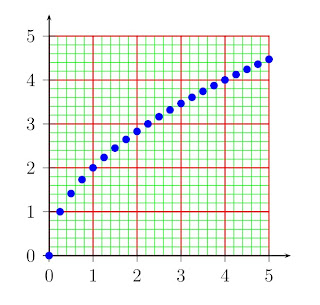
The first one is "\fileplot[parameters]{datafile}". The datafile should contain a list of coordinates. And the data can be delimited by "{}", "()", "," and one or more white space. If something is following "%", it will be interpreted as comments and will be omitted. It is advised to bracket all the data with "[]", this will significantly speed up the rate at which the data is read. So files like the following ones are all legal.

%mydata
[(0,0),(1,1),(2,2),(3,3),(4,4)] %mydata

[{0,0},{1,1},{2,2},{3,3},{4,4}]

[{0  0}  {1  1}  {2  2}  {3  3}  {4  4}]

[0  0  1  1  2  2  3  3  4  4]

Now a simple practice on this command will be shown.

\documentclass{article}
\usepackage{pst-plot}
\usepackage{pstricks}
\begin{document}
  \begin{pspicture}(-1,-1)(5.5,5.5)
    \psgrid[gridcolor=red,subgridcolor=green,
      gridlabels=0](0,0)(5,5)
    \psaxes{->}(0,0)(5.5,5.5)
    \fileplot[linecolor=blue,plotstyle=dots,
      dotstyle=*,dotsize=5pt]{mydata.dat}
  \end{pspicture}
\end{document}

File mydata.dat is shown below:

[{0.,0.},{0.25,1.},{0.5,1.41421},{0.75,1.73205},
{1.,2.},{1.25,2.23607},{1.5,2.44949},{1.75,2.64575},
{2.,2.82843},{2.25,3.},{2.5,3.16228},{2.75,3.31662},
{3.,3.4641},{3.25,3.60555},{3.5,3.74166},
{3.75,3.87298},{4.,4.},{4.25,4.12311},{4.5,4.24264},
{4.75,4.3589},{5.,4.47214}]

And the output picutre looks like this:

Fig.1 Plot data file with command fileplot.

Files Download: tex ps pdf

Other file plot commands will be talked next time.

Tuesday, December 13, 2011

How to plot using pstricks(1)----plot a function

After the previous posts, now we have the ability to deal with the plotting problems using pstricks. And this time we will talk about how to plot a function using pstricks.

The command used to plot a function in pstricks is "\psplot{xmin}{xmax}{function}". "xmin" and "xmax" determine the plot range and "function" is the function to be plotted. "function" should be written in postscript code. Since this blog is not about postscript, how to write a function in postscript code will not be talked in detail, only when it is used some simple explanation will be given.

There are also some optional parameters to control the appearance of the plot. "plotstyle=line,polygon,dots,curve..." controls the plotstyle, "plotpoints=int" controls how many points be plotted and other parameters such as "showpoints", "linestyle", "linecolor", "dotstyle"... have the same meaning as we have talked before.

Now we come to some examples.

\documentclass{article}
\usepackage{pst-plot}
\usepackage{pstricks}
\begin{document}
  \begin{pspicture}*(-1,-1)(5.5,5.5)
    \psgrid[gridlabels=0,gridcolor=gray,
      subgridcolor=lightgray](0,0)(5,5)
    \psaxes{->}(0,0)(0,0)(5.5,5.5)
    \psplot[linecolor=blue,plotstyle=dots,
      plotpoints=15,dotstyle=x,dotsize=4pt]
      {0}{5}{x}
    \rput{45}(2.5,3){\color{blue}$y=x$}
    \psplot[linecolor=red,plotstyle=dots,
      plotpoints=15,dotstyle=+,dotsize=4pt]
      {0}{5}{x 2 exp 5 div} %(x^2)/5
    \psplot[linecolor=red,plotstyle=line]
      {0}{5}{x 2 exp 5 div} %(x^2)/5
    \rput{55}(4,2.25)
      {\color{red}$y=\frac{x^{2}}{5}$}
    \rput(0.25,5.25){$y$}
    \rput(5.25,0.25){$x$}
  \end{pspicture}
\end{document} 

2
Fig.1 An example of Psplot—Plot function y = x and y = x /5.

\documentclass{article}
\usepackage{pst-plot}
\usepackage{pstricks}
\begin{document}
  \begin{pspicture}*(-1.25,-1.25)(4.5,1.25)
    \psgrid[gridlabels=0,gridcolor=red,
      subgridcolor=green](0,-1)(4,1)
    \psaxes[labels=y,tickstyle=bottom]
      {->}(0,0)(0,-1.25)(4.5,1.25)
    \rput(0.25,1){$y$}
    \rput(4.25,0.25){$x$}
    \psset{xunit=0.0111cm} %xuni=4cm/360
    \psplot[plotstyle=curve,
      linecolor=blue]{0}{360}{x sin}
       %"x sin" is postscript code
       %with meaing sin(x)
    \psplot[plotstyle=curve,linecolor=brown,
      linestyle=dashed]{0}{360}{x cos}
       %"x cos" is postscript code
       %with meaing cos(x)
    \uput[-90](90,0){$\frac{\pi}{2}$}
    \uput[-90](180,0){\scriptsize $\pi$}
    \uput[-90](270,0){$\frac{3\pi}{2}$}
    \uput[-90](360,0){\scriptsize $2\pi$}
  \end{pspicture}
\end{document}

Fig.2 Another example of Psplot—Plot function y = sin(x) and y =
cos(x).

Files Dowload: tex ps pdf

Sunday, December 11, 2011

Axes of coordinates

This posts will talk about making axes. Axes is an essential part in a plotting. And after this posts, I think we have gained enough knowledge to take over the subject of plotting. So in the next posts plotting will be talked about.

The command for drawing axes in pstricks is "\psaxes(x0,y0)(x1,y1)(x2,y2)" in package "pst-plot" (so do remember to include this package). (x0,y0) is the position of the origin. (x1,y1) is the lower left corner of the coordinate and (x2,y2) is the upper right corner. If (x0,y0) is not specified, (x1,y1) will be used. And if both (x0,y0) and (x1,y1) is not specified, then the origin of the current coordinate will be used. It is to say that "\psaxes(x1,y1)(x2,y2)" is equivalent to "\psaxes(x1,y1)(x1,y1)(x2,y2)" and "\psaxes(x2,y2)" is equivalent to "\psaxes(0,0)(0,0)(x2,y2)". Isn't it very similar to the command "\psgrid"?

As axes is in fact a line, the command "\psaxes" can take almost all the parameters a line can take. And there are also some parameters specially for it.

"Ox(y)=num" is the label at origin with default value 0. "Dx(y)=num" is the label increment with default value 1. "dx(y)=num" is the distance between labels. If it takes value 0, Dx*\psunit will be used, and the default value is 0. "labels/ticks=all/x/y/none" controls which labels/ticks will appear. "showorigin=true/false" controls whether the origin label will be drawn. "tickstyle" can take values "full","top" and "bottom". If "top" is chosen, the ticks are only on the side of the axes away from the label. "Bottom" is just the opposite. And "full" gives ticks on both sides of the axes. The size of the ticks can be set using parameter "ticksize". Another mostly used parameter is "axesstyle", its legal values include "axes","frame" and "none".

In the following example the using of "\psaxes" is illustrated.

\documentclass{article}
\usepackage{pst-plot}
\usepackage{pstricks}
\begin{document}
  \begin{pspicture}(5,5)
    \psaxes[axesstyle=frame,Ox=0,Oy=100](4,4)
  \end{pspicture}
  \hspace{1.5cm}
  \begin{pspicture}(5,5)
    \psframe[linecolor=lightgray](0,0)(5,5)
    \psaxes[Dx=1,Dy=0.5,linewidth=1pt,
      ticksize=4pt]{->}(2,2)(0.5,0.5)(4.5,4.5)
  \end{pspicture}

  \vspace{1cm}

  \begin{pspicture}(5,5)
    \psframe[linecolor=lightgray](0,0)(5,5)
    \psgrid[gridcolor=red,subgridcolor=green,
      gridlabels=0](1,1)(1,1)(4,4)
    \psaxes[showorigin=false,
      tickstyle=bottom]{->}(1,1)(4.5,4.5)
  \end{pspicture}
  \hspace{1.5cm}
  \begin{pspicture}(5,5)
    \psframe[linecolor=lightgray](0,0)(5,5)
    \psaxes[axesstyle=frame,
      showorigin=false](5,5)(5,5)(1,1)
  \end{pspicture}
\end{document} 

Fig.1 The usage of Psaxes
Files Download: tex ps pdf

Thursday, December 8, 2011

A Powerful Pstricks Tool ---- Psgrid

Making grid with pstricks is very easy. You can just include "\psgrid" in your pspicture environment (note that psgrid can also used outside pspicture environment), then a beautiful grid will be drawn, just like the following:

\documentclass{article}
\usepackage{pstricks}
\begin{document}
  \begin{pspicture}(5,4)
    \psgrid
  \end{pspicture}
\end{document}

Fig.1 The simplest usage of psgrid

Command "\psgrid" can be followed with three arguments, i.e., "\psgrid(x0,y0)(x1,y1)(x2,y2)". (x1,y1) and (x2,y2) are the opposing corner of the grid area. The dedault value of (x1,y1) is (0,0). If (x1,y1) and (x2,y2) are both not specified, in a pspicture environment the coordinate of the current pspicture will be used, and outside a pspicture environment (10,10) will be used. By default, the intervals are labeled. The horizontal labels will be placed at positions (*,y0) and the vertical labels will be placed at positions (x0,*). If (x0,y0) is omitted, (x1,y1) will be used.

The appearance of the grid can be changed if some parameters are applied."(sub)gridwidth","(sub)gridcolor" can be used to change the width and color of the main grid and sub grid. When (sub)griddots=num and num is a positive value , the (sub)grid lines are dotted with num dots per division. gridlabels and gridlabelcolor can used to control the size and color of the grid lables, and the default value of these two parameters is 10pt and black. If a positive int number(num) is set to parameter subgriddiv, then the main grid will be divided into num parts, and the default value is 5.

In the following example we will examine "\psgrid" in detail.

\documentclass{article}
\usepackage{pstricks}
\begin{document}
  \begin{pspicture}(9,9)
    \psgrid[gridcolor=red,subgridcolor=green]
      (1,5)(1,5)(4,8)
    \psgrid[gridcolor=blue,subgridcolor=yellow,
      gridlabels=5pt](6,6)(5,5)(8,8)
    \newrgbcolor{mycolor1}{0.5 0.3 0.3}
    \newrgbcolor{mycolor2}{0.3 0.5 0.5}
    \psgrid[gridcolor=mycolor1,
      subgridcolor=mycolor2,subgriddiv=2,
      subgridwidth=0.8pt,subgriddots=15,
      gridlabels=0](1,1)(4,4)
    \psgrid[griddots=10,subgriddots=3,
      gridlabelcolor=red](5,1)(8,4)
  \end{pspicture}
\end{document}

Fig.2 Psgrid with some options
Files Download: tex ps pdf

Tuesday, December 6, 2011

Some basic graph objects in pstricks (4) ---- Curves

There are several commands for curve drawing in Pstricks. "\psbezier" draws a Bezier curve, "\parabola" draws a parabola, and "\pscurve", "psecurve", "psccurve" interpolate curves through the given points. In the following they will be introduced one by one.

Bezier curve is really a set of curves (Linear Bezier curve, Quadratic Bezier curve, Cubic bezier curve ...). The Bezier curve in Pstricks is cubic Bezier curve. And to to determine a cubic Bezier curve four control points are needed ("How to draw a cubic Bezier curve according to four given points" can be found in Wikipedia). So the complete form of "\psbezier" is "\psbezier [parameters] {arrowtype} (x0,y0)(x1,y1)(x2,y2),(x2,y3)".

"\parabola [parameters] {arrowtype} (x0,y0)(x1,y1)" draws a parabola with maximum or minimum (x1,y1) staring from (x0,y0).

"\pscurve [parameters] {arrowtype} (x1,y1)...(xn,yn)" interpolates an open curve through the given points. "\psecurve" is similar to "\pscurve" except that the curve is not extend to the first and last points. "\psccurve" draws a closed curve.

The curvature of a curve is controlled by the parameter "curvature".

Now we use these commands to draw several curves.

\documentclass{article}
\usepackage{pstricks}
\begin{document}
  \begin{pspicture}(5,5)
    \psset{showpoints=true}
    \psbezier[linecolor=green]
      (0,0)(0,3)(5,1)(5,5)
    \parabola[arrowsize=10pt]
      {->}(5,5)(2.5,0)
    \pscurve[linecolor=red]
      (0,4)(1.25,5)(2.5,4)(3.75,3)(5,4)
    \pscurve[linecolor=blue,
      curvature=0.5 0.1 0]
      (0,1)(1.25,0)(2.5,1)(3.75,2)(5,1)
    \psccurve[fillstyle=solid,
      fillcolor=yellow]
      (3,4)(4.5,4)(4.5,4.5)(3,4.5)
  \end{pspicture}
\end{document} 

Fig.1 Draw Curves using Pstricks
Files Download: tex ps pdf

Sunday, December 4, 2011

Some basic graph objects in pstricks (3) ---- Circles,Arc,Wedge,Ellipses,Elliptic Arc,Rectangle and so on

"\pscircle[parameters](x0,y0){r}" draws a circle whose center is located at (x0,y0) and that has radius r.

"\pswedge[parameters](x0,y0){r}{ang1}{ang2}" draws a wedge whose center is located at (x0,y0), that has radius r and extened counterclockwise from ang1 to ang2.

"\psarc[parameters]{arrowstyle}(x,y){r}{angA}{angB}" clockwisely draws an arc form angA to angB. (x,y) and r are the center and radius of the circle ( a arc curve is always a part of a circle).

"\psellipse[parameters](x0,y0)(h_r,v_r)" draws a ellipse. (x0,y0) is the center, h_r is the horizontal radius and v_r is the vertical radius.

"\psellipticarc[par]{arrow}(x0,y0)(x1,y1){angA}{angB}" which is very similar to "\psarc" draws an elliptic.

"\psframe[parameters](x0,y0)(x1,y1)" draws a rectangle with lower left corner at (xo,y0), upper right corner at (x1,y1).

There are also command like "\pstriangle","\psdiamond" to draw triangle and diamond. But we can use "\pspolygon" to realize the utility of all these commands. So we will not talk about them here.

For all these commands a star can be followed (for example, "\pscircle*"). This determine the fill the object.

Now let we have a practice on these commands.


\documentclass{article}
\usepackage{pstricks}
\begin{document}
  \begin{pspicture}(-2.5,2.5)(2.5,2.5)
    \psframe[linestyle=none,framearc=0.25,%
      fillstyle=solid,fillcolor=green]
      (-2.5,-2.5)(2.5,2.5)
    \pscircle[linecolor=red](0,0){2.5}
    \pswedge[fillstyle=solid,
      fillcolor=red](0,0){2.5}{0}{45}
    \psarc{->}(0,0){1.5}{0}{45} %draw arc
    \uput{1.5}[22.5]
      (0,0){$45^{\circ}$} %put a label
    \psellipse(0,-1.25)(2.5,1.25)
  \end{pspicture}
\end{document}

This practice draw something like this:

Fig.1 Draw circle,arc,ellipse,rectangle... uisng Pstricks
 Files download: tex ps pdf

Thursday, December 1, 2011

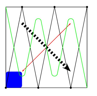
Some basic graph objects in pstricks (2) ---- Lines

Command "\psline[parameters]{arrowstyle}(x1,y1)(x2,y2)...(xn,yn)" draws a line through points (x1,x2),(x2,y2)...(xn,yn).

Command "\pspolygon" is similar to "\psline", except that it draws a closed path and when a star is added, the closed area is filled with linecolor.

Arrowstyle can be specified to tell pstricks which type of arrowhead the line terminated. The most used parameters include "linecolor", "linewidth", "linestyle" "linearc" and "cornersize". Linecolor and linewidth have the its literal meanings. Linestyle can take values "none,solid,dashed,dotted". When "dashed" is used, paramter "dash=len1 len2" can be used to specify the dash pattern. And when "dotted" is used, paramete "dotsep=len" can be used to specify the distance between the nearest two dots. If you want the line have round corners, parameter "linearc" is very useful. This parameter specifies the radius of arcs drawn at the corners. To show the points on the line, "showpoints=true" can be useful. To show how these commands and parameters are used, there is an example.

\documentclass{article}
\usepackage{pstricks}
\begin{document}
  \begin{pspicture}(5,5)
    \pspolygon(0,0)(5,0)(5,5)(0,5)
    \pspolygon*[linestyle=none,linecolor=blue,
      linearc=4pt](0,0)(1,0)(1,1)(0,1)
    \psline[linecolor=red,linestyle=solid]
      {<->}(1,1) (4,4)
    \psline[linewidth=5pt,linestyle=dashed,
      dash=3pt 3pt]{->}(1,4) (4,1)
    \psline[showpoints=true]
      (0,0)(1,5)(2,0)(3,5)(4,0)(5,5)
    \psline[linearc=5pt,linecolor=green]
      (0,5)(1,0)(2,5)(3,0)(4,5)(5,0)
  \end{pspicture}
\end{document}

The lines looks like this:
Fig.1 Lines drawn using Pstricks
Files Download: tex ps pdf


Creative Commons License
Except as otherwise noted, the content of this page is licensed under a Creative Commons Attribution-NonCommercial-NoDerivs 3.0 Unported License.